Databases
In addition to preparing a geometric model, a lot of data is required for the calculation, such as: thermophysical and mechanical properties of materials and alloys, heat transfer parameters between bodies and with the environment, temperature, speed conditions, etc. Some of this data: material properties and heat transfer parameters, is mandatory for any calculation; others are used depending on the case. Editing, storage and other operations with this data are performed in the same type of editors, a description of which is given below in the relevant sections.
Data Editors. General Controls and Features
The material properties, boundary conditions and other data editors, despite the fundamental differences, have the same interface. The window of any editor contains a toolbar (1), a table of editable parameters (2) and an area for editing curves (3) (see the figure below). If there is a * symbol at the end of the editor's caption, it means that the parameters have been changed. When you close the editor, you will be prompted to save your changes.
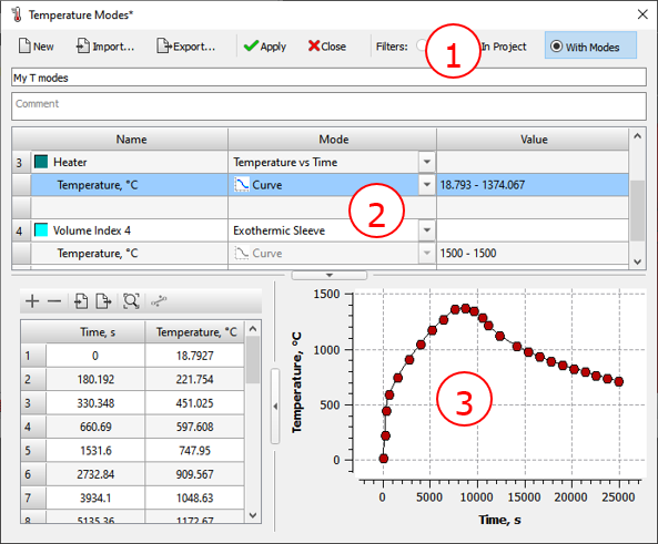
Temperature Modes Editor
Under the toolbar (1) there is a line where you can enter the name of the data set. This name will then be displayed in the corresponding line in the parameters table (Start Simulation and Parameters window). Below is a line for entering a comment on the data set.
Further in this section, interface elements and buttons common to all editors are considered. The following sections give more detailed descriptions of all editors and the data edited in them.
Toolbar Buttons
All editors have a toolbar at the top with buttons for general data operations (see figure below).

Temperature Modes Toolbar
 |
The New button creates a new data set with "default" parameters. The data is created for use in the current project. |
 |
The Import button opens a standard dialog for loading data into the project. It is possible to import data created in older versions of PoligonSoft. |
 |
The Export button export data from the project to files that can form a user database and then be used in other projects. This command is also used if you want to save edited data in the original file. |
 |
The Apply button saves the imported or/and edited data in the project. The original data file remains unchanged. To update it, use the Export button. |
 |
The Close button closes the editor. If the data in the editor has been changed, a message will be displayed asking you to save it. |
On the right side of the toolbar are filters that change the set of displayed data. The operation of filters depends on the nature of the displayed data, so their operation is discussed in the relevant sections below.
Editing Constants and Functions
Many material characteristics and simulation conditions can be specified either by constants or by curves. In this case, the drop-down list is active in the parameters table, in the Mode column (see the figure below).

Editing the ambient temperature in the Heat Transfer Editor
If Value is selected, then the parameter should be set as a constant in the Value column. If Curve is selected, the curve editing area at the bottom of the editor becomes active. It contains: on the left - a table with coordinates of points and a toolbar for working with a curve; on the right is the curve drawing area (see the figure below).
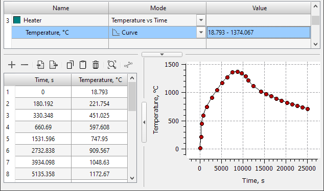
Curve Editing Area
Above the table with the coordinates of the curve points there is a toolbar with buttons that control the data in the table.
 |
The Add Row button creates a new row in the table. The row is created under the current (active) table row. New row cells default values based on the values set in the previous and next cells. At the same time, a new point is displayed in the curve drawing area, it is highlighted in yellow. |
 |
The Delete Row button deletes the selected row in table. |
 |
The Import Curve Points button opens a standard dialog for loading data into a table. It is possible to import data from .csv (MS Excel), .lin (PoligonSoft) files and any other text files containing curve points in the "x y" format. |
 |
The Export Curve Points button exports the data from the table to a .lin text file (PoligonSoft) that contains the curve points in the "x y" format. The file can be imported into other spreadsheet editors such as MS Excel. |
 |
The Copy Table button copies the table to the clipboard. The data can be pasted into another table or into another application. |
 |
The Paste Table button pastes data from the clipboard. |
 |
The Delete Table button deletes all table rows. To delete one or more selected table rows, use the  button. button. |
Editing the table results in an immediate change in the appearance of the curve in the drawing area on the right. The curve must contain at least two points. The table of editable parameters will display the minimum and maximum values of the parameter.
The drawing area is interactive, the user can change the appearance of the curve and edit it with the mouse.
- Clicking the left mouse button on a point highlights it in yellow. At the same time, the corresponding row in the table is highlighted. You can select any number of points by clicking on them with the mouse and holding down the Ctrl button on the keyboard.
- The selected point can be moved by holding down the left mouse button. At the same time, the values of the coordinates of the point in the corresponding line of the table change.
- By holding down the left mouse button, you can move the entire curve over the drawing area.
- Using the mouse wheel, you can change the scale of the curve display.
 |
The Fit button returns the curve display to its default state. |
 |
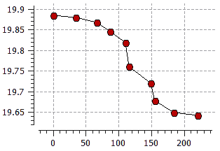
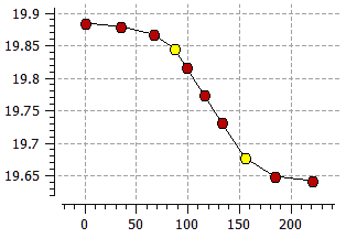
The Line button allows you to create a linear section of the curve between two selected points. When two points are selected, the button becomes active. On fig. below is an example of how this command works. |
|
|
|
Initial curve |
Curve with linear section |
Example of creating a linear section of a curve
Material Properties
The Material Properties editor (see figure below) is used for creating and editing materials used in the calculation. Materials are stored in the %PoligonSoft%\Database folder in pmat files (older versions have bd, fil and bdd extensions). Each material must contain a set of characteristics required for PoligonSoft solvers: Euler, Fourier, Hooke, etc.
 |
The button to launch the Material Properties editor is located on the Process toolbar and on the Main tab of the ribbon menu. The editor can also be opened from the Materials tree on the Project Overview tab and from the Start Simulation and Parameters window. See Materials Assignment section for more details. |
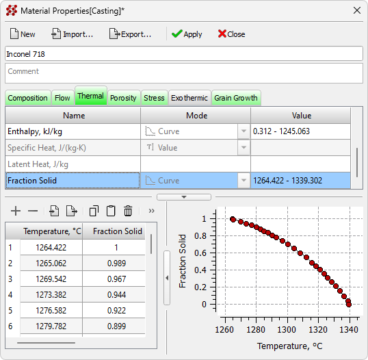
Material Properties Editor
Under the toolbar there is a line with the name of the material, which can be changed. The comment box is located below. The following is a table of material properties, with properties divided into tabs:
- Composition;
- Flow;
- Thermal;
- Porosity;
- Stress;
- Exothermic;
- Grain Growth.
Tabs can be of three colors (see the figure below): gray - the tab does not contain data; green - the tab contains the minimum set of material properties that are sufficient to run the solver; pink - the set of properties is not enough to run the solver.

Different tabs colors
On the tab marked in pink, the properties that are not set but required to run the solver are also highlighted in pink (see the figure below).
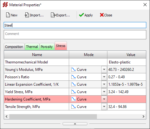
Highlighting undefined properties
The ability to import material properties in a legacy format is retained. Older versions of materials have the extensions bd (thermal properties), fil (shrinkage properties) and bdd (mechanical properties). When importing a bd (thermal properties) file, other file types with the same name are searched. If other alloy properties are found, the Master offers to load them into the appropriate tabs (see the figure below).
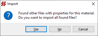
Message suggesting importing material properties
When importing fil (shrinkage properties) and bdd (mechanical properties) files, the properties are loaded into the respective tabs, but other file types are not searched.
Composition Tab
The tab contains a table of chemical composition (see figure below). In the first line of the table, you can select the base element of the alloy (Fe, Al, Ni, Ti, etc.) and then enter the content of the remaining elements in weight percent.
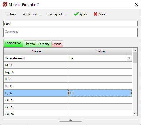
Material Properties, Composition Tab
The tab turns green if the content of at least one chemical element or a basic element is specified in the table.
The data in this tab can be used as input for the Heat Treatment solver (for more details see the Heat Treatment Simulation) section).
Thermal Tab
The tab contains a set of material characteristics required to calculate the temperature and phase fields (see the figure below). To calculate temperature fields in bodies where there is no phase transition (usually it is a mold), the minimum set of thermophysical properties required for calculation includes:
- Thermal conductivity;
- Specific heat;
- Density.
These properties can be specified either as constants or as functions of temperature.
In the presence of a phase transition, i.e. solidification (usually these are bodies of the “casting” type), you should additionally specify the following characteristics:
- Latent Heat;
- Fraction of Solid.
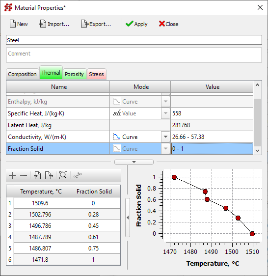
Material Properties, Thermal Tab
The Solid Fraction is a function of temperature. Its values should start from 0 at the liquidus temperature and increase to 1 at the solidus temperature. Thus, the fraction of the solid phase is determined by a falling curve strictly between 0.0 and 1.0. Isothermal transformation (for example, eutectic) is recommended to be "stretched" by an interval, for example, of 2-3 degrees. Latent Heat is given by a constant.
It should be noted that the PoligonSoft algorithms allow you to set the fraction of the solid phase with flat sections. The recommendation to "stretch" them by 2-3 degrees is not mandatory.
An alternative way of defining the phase transition is possible. Instead of Specific Heat and Latent Heat, the corresponding Enthalpy curve can be given as a function of temperature H(T), which is defined as follows:

where cp(T) – Specific Heat;
Q – Latent Heat;
fs(T) – Fraction of Solid.
Since there are two ways for defining a phase transition, the editor automatically avoids conflict between the following options:
- Specific Heatcp(T);
- Latent Heat Q;
or
- Enthalpy H(T).
If specific heat or latent heat is entered, the enthalpy entry is blocked, and vice versa.
Thermal conductivity and enthalpy must always be given as a temperature curve.
Porosity Tab
The tab contains a set of material properties needed to calculate pipe shrinkage, macro- and microporosity in a casting (see the figure below).
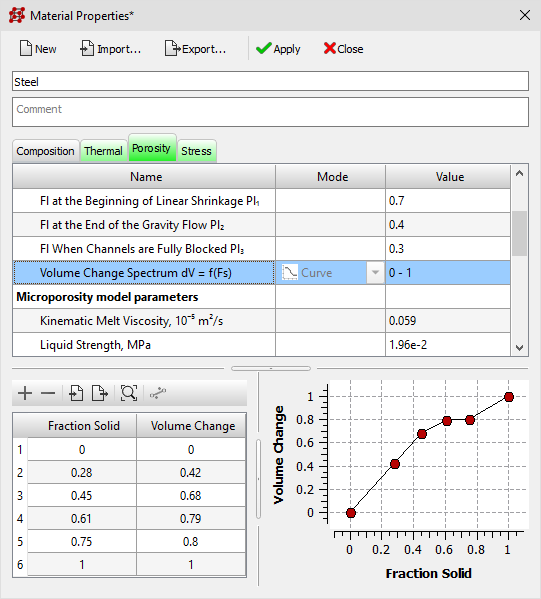
Material Properties, Porosity Tab
The set of parameters required for the "standard" macroporosity model used in PoligonSoft:
- Melting Volume Change;
- Liquid Phase Volume Change;
- Pl1 – fraction of liquid phase at the beginning of linear shrinkage;
- Pl2 – fraction of liquid phase at the end of the gravity flow;
- Pl3 – fraction of liquid phase when channels are fully blocked;
- Volume Change Spectrum dV = f(Fs).
To calculate microporosity according to the "standard" PoligonSoft model, in addition to the parameters listed above, it is required to set the parameters:
- Kinematic Melt Viscosity;
- Liquid Strength.
To calculate the filtration coefficient using the equation:
 ,
,
| where |  |
fL и fs – fractions of liquid and solid phases, respectively;
λII – secondary dendrite arm spacing
need to define:
- coefficient Ко;
- power n.
At the end of the table, the set of parameters required for the new porosity model is listed, which extends the capabilities of the "standard" macro- and microporosity models:
- Fraction of liquid phase at the beginning of linear shrinkage;
- Fraction of liquid phase when channels are fully blocked;
- Critical Pressure Pcrit;
- Melt Compressibility Modulus E;
- Surface Tension Coefficient σ;
- Secondary Dendrite Arm Spacing λII.
Some parameters from this list duplicate the parameters of the "standard" macroporosity, but nevertheless must be set again. This is because the parameter values are different when used in different models and their separation is convenient for switching between new and standard porosity models.
For more information on the new model of porosity and its parameters, see the New Pipe Shrinkage and Macroporosity Model section.
Stress Tab
The tab contains a set of material properties required to calculate the stress-strain state of the casting and the mold (see the figure below).
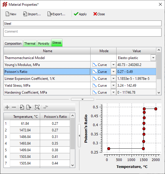
Material Properties, Stress Tab
Different stress models can be used in the calculation, each requires its own set of mechanical characteristics. The stress model is selected from the list, which is located in the first line of the parameter table. The following options are available:
- Linear Elastic;
- Elasto-plastic.
The Linear Elastic model is characterized mainly by Young's Modulus. In addition, the Poisson's Ratio and the Thermal Expansion Coefficient must also be specified. The value of Poisson's Ratio for metals is approximately 0.3.
For an Elasto-plastic model, the properties described above for an elastic model, i.e. Young's Modulus, Poisson's Ratio and Thermal Expansion Coefficient must also be given. In addition to this, the Yield stress and Hardening Coefficient must be specified.
All listed properties can be specified by constants or temperature curves. Of course, it is extremely undesirable to set the properties with a constant, since in this case the accuracy of the calculation decreases. For example, if all properties are given by constants, then the result of the calculation will in no way depend on the change in the temperature field of the casting and the mold.
The source of stress properties can be: literature, the Internet and scientific research. If these sources cannot provide the necessary data, then they can be obtained empirically, i.e. by carrying out the necessary mechanical tests.
Exothermic Tab
The tab contains a set of parameters (see the figure below) necessary for heat release simulation when using mold elements made of exothermic (thermitic) mixtures (sleeves, covers, mats, etc.). Such a material must be specified in the model as a separate volume of the “mold” type with the necessary thermophysical properties are specified on the Thermal tab (for more details see the Thermal Tab section). Then the required parameters for the exothermic reaction should be specified:
- Exothermic Energy. The amount of heat released by 1 kg of material during the period from the beginning to the completion of the thermite reaction.
Specified as an integer in kJ/kg - Burnt Fraction. Sets the total duration and rate of the reaction (see the figure below). Generaly, the reaction may proceed unevenly with time intervals of deceleration and acceleration of the process, which can be taken into account in the calculation.
It is given by a time - reaction fraction curve, where the time is given in seconds. - Ignition Temperature. The parameter sets the temperature of the thermite reaction (ignition), which "switch on" the calculation of heat release in the corresponding mesh node of the exothermic material.
Specified as an integer in Celsius.
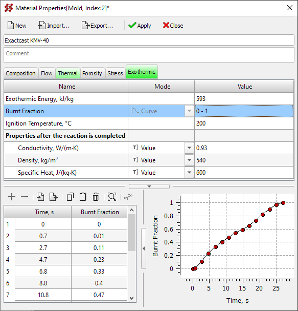
Material Properties, Exothermic Tab
If at least one of the three parameters described above is not set, the tab will be colored pink. This means that there is not enough data to run the calculation. The corresponding parameter lines will also be pink. If all parameters are set, the tab is colored green.
Additionally (but not necessarily) the thermophysical properties of the material after completion of the reaction can be specified. They differ from the initial exothermic material properties, specified on the Thermal tab, and can be used in the calculation to take into account the heat-insulating ability of burnt material. The following properties will be used when calculating temperatures for those mesh nodes where the burnt fraction is equal to 1:
- Conductivity;
- Density;
- Specific Heat.
These properties can be specified by constants, or temperature curves. All three properties must be set. If the properties of the material after the completion of the reaction are not set, then properties from the Thermal tab will be used for the heat transfer calculation in the areas, where the fraction of burnt material is equal to 1.
When using exothermic materials, it may be necessary to enter specific heat transfer parameters at the casting-material and material-mould interfaces. These parameters are set in the Heat Transfer editor (see the Heat Transfer Parameters section). For more information on modeling foundry technology using exothermic materials, see the Exothermic Sleeves section.
Grain Growth Tab
The tab contains coefficients determined by the chemical composition of the alloy, which are used in the equation for the growth rate of the primary axis of the dendrite in the grain growth model (see figure below). This data is used by the Macrostructure solver. For more information about macrostructure simulation, see the Macrostructure Simulation section.
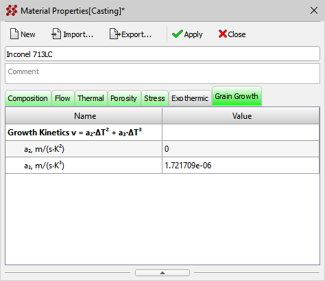
Material Properties, Grain Growth Tab
Heat Transfer Parameters
The Heat Transfer editor is designed to create and edit heat transfer settings at the boundaries between volumes (Body-to-Body) and at the outer boundaries (Body-Environment). The settings can be applied to solve one specific problem or exported to a file with the afo extension for use in other calculations, including as a casting process template.
 |
The button to launch the Heat Transfer editor is located on the Process toolbar and on the Main tab of the ribbon menu. The editor can also be opened from the Start Simulation and Parameters window. |
The table, which occupies the upper part of the editor, specifies the heat transfer conditions for all surfaces of each volume of the computational domain. The heat transfer parameters for each surface (boundary) are determined by a specific task and depend on where this boundary is located. Regardless of the problem being solved, the table always contains data on all 18 boundaries, which in general can all be specified in the model (for more details see Basic concepts: Volumes, Types, indices section). There is no boundary at index 0 in the boundary list because it is an internal border and does not require any parameters to be specified. To display in the table only those boundaries that are specified in the model, you can use the In Project filter located on the toolbar (see the figure below). Use the All filter to display the entire list of boundaries.
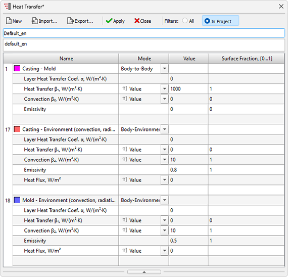
Heat Transfer Editor, In Project filter
The list of heat transfer parameters for each boundary begins with a line that specifies its index and color, which is used for visualization in the pre- and postprocessor in the boundary indices mode. In the same line, in the Name column, you can enter an explanatory text describing, for example, the heat transfer conditions. This text will be displayed in preprocessor dialogs when editing boundaries. The next column Mode indicates one of the two heat transfer modes. For boundaries with indices 1-9, it can be changed. Сlicking on a line brings up a drop-down list in which you need to select the desired option (see the figure below):
- Body-to-Body mode sets the heat transfer between the casting and the mold, or between different parts of the mold. In this mode, heat is transferred across a selected boundary from a body with a higher temperature to a body with a lower temperature. It is assumed that the boundary with this index (and this color) is set on the contact surfaces of both bodies. If in the computational domain one of the outer surfaces of the body has a boundary for which this mode is specified, but the second body is absent, then the heat transfer will go between the real and the virtual body. For example, if the boundary with this mode is set on the outer surface of the casting, and the body of the mold is absent, then the heat transfer will go into a virtual mold of infinite thickness. In this case, the thermal activity of the mold will be taken into account (the root of the product of the volumetric heat capacity and thermal conductivity). The characteristics of the mold material from the specified set of mold materials with an index equal to the boundary index will be used. For more information on the virtual mold, see the Virtual Mold section.
- Body-Environment mode sets the heat exchange between the volume (casting or mold) and the environment with a given temperature.

Changing the heat transfer mode for the boundary
As indicated in the Basic concepts: Volumes, Types, indices section, the first nine boundaries, starting from index 1, are universal and can be used as boundaries between bodies of the computational domain or as external boundaries with the environment. All other boundaries with indices 10-18 set the parameters of heat transfer between the body and the environment.
In the Body-Environment boundary mode, the Ambient Temperature, °С line becomes available.The ambient temperature can be set by a constant value or by a temperature-time curve. To select, you need to click the left mouse button in the Mode column and select the desired option from the drop-down list (see the figure below).

Editing the ambient temperature for the boundary with index 2
If the ambient temperature is constant, select the Value mode and set the temperature in the next cell Value. If the ambient temperature changes depending on time, select the Curve mode. In this case, the table and the curve drawing area in the lower part of the editor window become active, where you can set the points of the curve in the temperature-time coordinates (see the figure below). For more information on editing curves, see the Editing Constants and Functions section.
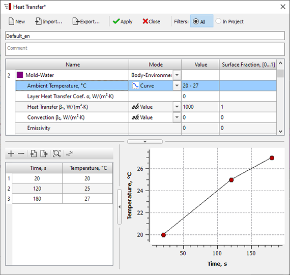
Ambient Temperature curve
It should be note in mind that for boundaries 17 and 18, the ambient temperature is set by a constant in the Start Simulation and Parameters window.
The next four lines set the heat transfer parameters, in accordance with the PoligonSoft model . This model can be represented as a scheme (see figure below) and describes three mechanisms of heat transfer: heat conduction, convection and radiation.
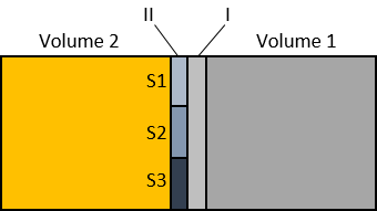
Scheme of the heat transfer model in PoligonSoft
It is assumed that, in the general case, at the boundary between volume 1 and volume 2, two successive layers can exist: let us designate them as I and II. Layer I is characterized by the heat transfer coefficient of the layer α, which is set by the user. For example, this could be a coating applied to a mold. If the thermal conductivity of the coating material λI and its thickness δ are known, then the heat transfer coefficient of the layer α can be calculated by the equation:
 |
(1) |
Layer II is characterized by a calculated heat transfer coefficient β. In general, the contact between volumes 1 and 2 is not ideal. It is assumed that heat transfer in layer II can take place in three ways: heat transfer in the zone of direct contact of volumes, convection and radiation where there is no contact. Each mechanism acts on a part of the boundary, which is specified by the relative areas S1, S2 and S3 respectively. Thermal conductivity and convection are given by the heat transfer coefficients (let's call them β1 and β2). The radiation is characterized by a given emissivity E. Then the calculated heat transfer coefficient β can be calculated as:
 |
(2) |
|
where |
Knowing the coefficients α and β, one can write down the equation for a heat flux density:
 |
(3) |
|
where |
At the outer boundaries of volumes, heat transfer in the general case can be carried out by heat transfer, convection and radiation. In addition, a constant heat flux can be specified at the outer boundary. The heat flux density in general is determined by the expression:
|
|
(4) |
|
where q – heat flux; |
Using the described model, the user can specify any mechanism for transferring heat from body to body or from body to environment. The following lines are used for this:
- Layer Heat Transfer Coef. (α, W/m2/K). This row specifies the heat transfer coefficient of the layer α, which can be used to account for the effect of the non-stick coating of the mold. It can be calculated using the formula (1). Specified by a constant value in the Value cell. If you set the parameter to 0, it will mean that layer I is missing.
- Heat Transfer (β1, W/m2/K). The line specifies the heat transfer coefficient βI, which then participates in the calculation of the total coefficient according to the formula (3). This parameter can be used to define the heat transfer between two bodies (for example, a casting-mold). Set as a constant value or curve by selecting the appropriate mode. A constant coefficient is set in the Value cell, the curve can be set in the lower part of the window. In the cell Surface Fraction, [0 ... 1] it is indicated which part of the surface is involved in heat exchange: 0 - does not participate; 0.5 - 50% percent of the surface is involved; 1 - the entire surface is involved.
- Convecton (β2, W/m2/K). The line specifies the heat transfer coefficient βII, which then participates in the calculation of the total coefficient according to formula (3). The parameter can be used to define heat transfer at the outer boundary (for example, mold-environment).. Set as a constant value or curve by selecting the appropriate mode. A constant coefficient is set in the Value cell, the curve can be set in the lower part of the window. In the cell Surface Fraction, [0 ... 1] it is indicated which part of the surface is involved in heat exchange: 0 - does not participate; 0.5 - 50% percent of the surface is involved; 1 - the entire surface is involved.
- Emissivity. The line specifies the emissivity E, which then participates in the calculation of the total coefficient according to formula (3). The parameter can be used to define radiation at the outer boundary (for example, mold-environment). Specified by a constant value in the Value cell. In the cell Surface Fraction, [0 ... 1] it is indicated which part of the surface is involved in heat exchange: 0 - does not participate; 0.5 - 50% percent of the surface is involved; 1 - the entire surface is involved.
- Heat Flux, W/m2. In some cases, it is necessary to specify the heat input or loss across the boundary as a given heat flow. The heat flow can be specified by a constant value or a temperature-time curve. Heat input across the boundary is specified by a positive value, and heat loss by a negative heat flow value. The line is only available in the Body-Environment boundary mode.
To switch off one or two heat transfer mechanisms from the calculation, it is necessary to set the corresponding fraction of the surface equal to 0. At least one of the three mechanisms of the second layer must be enabled.
For the procedure for saving heat transfer parameters and descriptions of other buttons located on the panel, see Toolbar Buttons section.
Data from files of outdated formats that were used in previous versions of PoligonSoft can be imported into the editor:
- files with afo extension with heat transfer parameters;
- files with qgr extension with heat flux data.
Temperature Modes
Temperature Modes editor is intended for creating and editing temperature modes of the casting and mold volumes. The settings can be applied to solve one specific problem or exported to a file with the .tel extension for use in other calculations. The ".tel" temperature file can be a part of a casting process template.
 |
The button to launch the Temperature Modes editor is located on the Process toolbar and on the Main tab of the ribbon menu. The editor can also be opened from the Start Simulation and Parameters window. |
In the table that occupies the upper part of the editor (see the figure below), temperature modes are set for all volumes of the model, for which you need to set special conditions that differ from those specified in the Start Simulation and Parameters window on the General tab (see deatils in Сommon Simulation Parameters section). Regardless of the problem being solved, the table always contains data on all 9 volume indices, which in general can all be specified in the model (more details about volume indices see in Basic concepts: Volumes, Types, Indices section). To display in the table only those volume indices that are specified in the model, you can use the In Project filter located on the toolbar (see the figure below). To display only volume indices with specified temperature modes, use the With Modes filter. Use the All filter to display the entire list of volume indices.
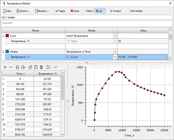
Temperature Modes Editor
For each volume index, the Name column contains the index, its color designation and explanatory text (name of the volume). In the next column Mode there is a switch for the set temperature mode. From the drop-down list it is proposed to select:
- [not assigned] – the temperature mode for the volume(s) is not set, the temperature for the volumes with this index will be assigned in the Start Simulation and Parameters window.
- Initial Temperature – the initial temperature of the volume(s) is set, which is different from the one specified in the Start Simulation and Parameters window.
- Temperature vs Time – the temperature of the volume(s) is given by a constant or a temperature-time curve. If the calculation time exceeds the time set for the last point of the curve, the temperature of the volume (s) remains equal to the temperature set for the last point of the curve.
- Temperature vs Time with Cutoff – the temperature of the volume(s) is set by the temperature-time curve. If the calculation time exceeds the time specified for the last point of the curve, the mode is "turned off", i.e. the temperature of the volume(s) begins to be calculated as usual.
Please note that the temperature set for the volume index will be applied to all volumes with this index regardless of their type (casting or mold). Pay attention to the temperature icons in the Model Tree to avoid mistakes.
The selected temperature mode is set in the Temperature line. This line is visible only if the temperature mode is set for the volume index. In the Initial Temperature mode, the temperature can only be set by a constant in the Value column. In the Temperature vs Time with Cutoff mode, the temperature can only be set by the curve in temperature-time coordinates.
If the Temperature vs Time mode is set, in the Mode column you can select one of the options: Value or Curve. If Value is selected, the temperature of the volume(s) of the selected index is set by a constant in the Value column. This means that the temperature in the volume(s) will be constant throughout the entire calculation
If the Curve option is selected, the table and the curve drawing area become active at the bottom of the editor, where you can specify the points of the curve in temperature-time coordinates. If the calculation time exceeds the time set for the last point of the curve, the temperature of the volume(s) remains equal to the temperature set for the last point of the curve. For more information on editing graphs, see the Editing Constants and Functions section.
For the procedure for saving temperature modes and descriptions of other buttons located on the panel, see Toolbar Buttons section.
Electrical Properties
The dialog box "Electrical Properties" is intended for creating and editing the files with the TOK extension containing the information about the electrical properties of the alloy and the specified parameters for calculating the electric heating.
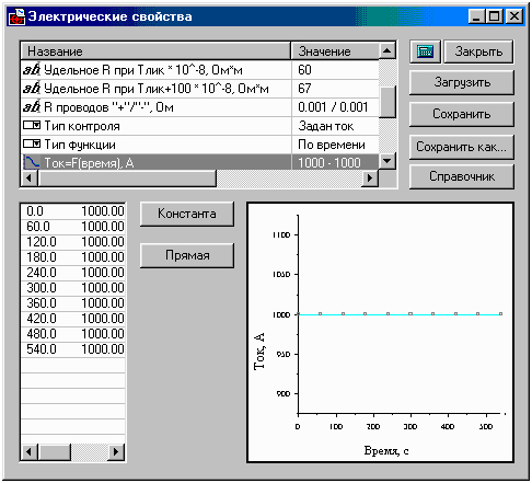
Electrical Properties Editor
The table of the properties and the parameters at the top of the dialog box opens with a line containing the "Write the potential file" switch. Double-clicking on the switch line results in a drop-down list in the “Value” column that consists of two positions: "Yes" and "No". Selecting the "Yes" position means that the calculation of the electric potential fields in the casting will be saved as a separate file.
The next line "The supply limits "+"/"-" is intended to indicate the indices of those casting boundaries through which an electric current is supplied to it. The boundary indices are placed in the “Value” column by the symbol "/".
Then there are four lines, in which the data characterizing the dependence of the resistance of the casting material on temperature are entered. This dependence is built on four reference points, the abscissas (temperature values) of which have the following values:
- The temperature of the colt solid metal – room temperature = 20°С;
- Solidus temperature;
- Liquidus temperature;
- The temperature of the liquid metal – for 100°С above the liquidus temperature.
When calculating, it is assumed that the resistivity between these points varies linearly. The values of resistivity at these temperatures are entered in the column "Value".
In the line "R wires "+"/"-"" you can specify the resistance of the lead wires. This can be important if the heating process is controlled by the voltage, and the voltage drop in the wires significantly affects the value of the actual stress on the casting. The resistance of the positive and negative wires is placed in the column "Value" through the symbol "/".
The "Control Type" line contains a parameter switch that determines what value will be used to monitor the electric heating process. Double clicking on the switch line results in a drop-down list of possible monitored values in the "Value" column:
- The voltage is specified – the current changes are not controlled;
- The current is specified – the voltage changes are not controlled.
The choice of the monitored value is carried out by selecting the required line in the drop-down list and then pressing the "Enter" key.
The "Function type" line contains a switch that determines, depending on which argument, the monitored value is changed assigned above. For example, you can specify that the heating current varies in a certain way as a function of time. And you can indicate that the heating voltage varies in a certain way, depending on the heat flow passing through a certain boundary of the model. The choice of the type of function (argument) of the process of electric heating is determined by the technological task you are solving and your approach to the simulation. The practical result of the calculation in this part is the development of an algorithm for the operation of an electric current source that would provide a given change in the controlled value depending on the change in the argument (control function).
Double-clicking on the switch line results in a drop-down list of possible monitoring functions in the "Value" column:
- By the time;
- By the flow through the boundary 1;
- ……………………………
- By the flow through the boundary 9.
Once you have determined the type of the monitored value and the type of monitoring function, you should specify this function, i.e. to construct a graph in which the values of the argument (control function) will be plotted along the abscissa axis and the values of the controlled quantity - along the ordinate. It is clear that the combinations of an argument / magnitude type can be only four. That why there is such quantity of the subsequent lines assigned to the setting the graphs of control functions:
Current = F(time);
Current = F(flow);
Voltage = F(time);
Voltage = F(flow).
You should select the appropriate line, double-click on it to open the necessary graph at the bottom of the dialog box and to edit it as described in the "Editing Constants and Functions" section.
The only selected dependency will be taken into account when you perform the calculation. The remaining dependencies will be present in the menu just only for decorative purposes.
Finally, in the last line of the "Note", double-clicking on it with the mouse, you can place any explanatory text you need for this file in the column "Value".
Dynamic Environment
The “Dynamic Environment” dialog box is intended for creating and editing the files with an AIR extension containing the information about the temperature modes of a multi-layer moving environment. A multilayer moving environment is a special situation in simulation that occurs, for example, in the process of directional crystallization of a casting. In this case, in contrast to the standard crystallization conditions, various parts of the mold get in contact with the layers of the external environment having different temperatures. This can be visualized in the form of a children's pyramid, where the casting in the mold plays the role of a toy rod, and the rings placed on top of each other represent the layers of the dynamic environment. On top of that, all these rings are moving along the rod in time.
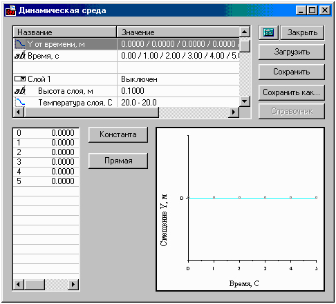
Dynamic Environment Editor
The first line Note opens the parameters table at the top of the dialog box.
The next two lines Y from time and Time specify the dynamics of the process of layers moving. In the Time line, you can arbitrarily set 6 time points (in seconds, from the start of the calculation) for which you will then specify the coordinates of the "tower" from the layers (in meters, relative to the selected zero point) in the Y from time line. The reference time points are entered in the Value column of the Time line through the "/" symbol, as described in the Alloy module editor. The main functions.
Then, in the Y from time line, you define the dependence of the ordinate of the layers on time, as described in the section Editing Constants and Functions. Naturally, the abscissas of the graph points correspond to the times previously set in the Time line.
Next, you should describe each of the necessary temperature layers. Such layers can be five. Accordingly, there are five same groups of rows - one for each layer in the parameters table.
The group consists of three lines. The first line contains the layer number and at the same time is a switch that allows you to enable or disable this layer when performing the calculation. Switching off the layer can be useful, for example, if the oven used for zone heating is not solid and has a height breaks. The second line is used to specify the height of the layer in meters. Finally, the third line is used to set the schedule for changing the temperature of the layer in time in accordance with the rules described in the section Editing Constants and Functions.
In this case, the abscissas of the graph points are already predefined programmatically and correspond to the time points previously set in the Time line.
Translation Modes
When modeling some foundry processes, it is necessary to take into account the movement of casting and/or mold volumes. For example, when simulating vacuum casting, you may need to take into account the movement of the mold within the furnace. To create and edit volume movements, use the Translation editor and the Translations tree in the Project Overview panel. Translation modes can be configured and used to solve one specific problem, or imported (and exported) into the project from files with the pmov extension (importing files of older versions with the mve extension is also supported).
 |
The Translation editor button is located on the Process toolbar and on the Main tab of the ribbon menu. The editor can also be opened from the Translation tree on the Project Overview tab (see the figure below). |
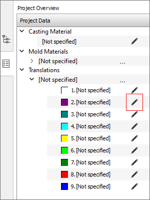
Buttons for opening the Translation editor in the tree in the Project Overview panel
The editor title indicates the volume index the translation mode will be created for, for example, in Fig. Below is the editor for moving volumes with index 2. Please keep in mind that the specified mode will be applied to all volumes with index 2, regardless of their type (casting or mold). If the translation mode has not yet been specified, then the editor looks like in the Fig. below, all interface elements are inactive. To start working in the editor, you need to create a translation mode for the selected index - click the New button.
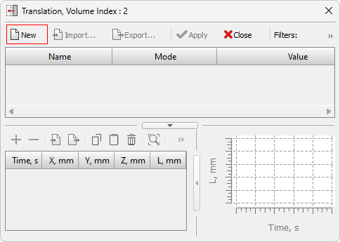
Translation editor
Unlike other editors, the Import and Export commands are inactive here, because these operations are performed through the Translations tree. Otherwise, the principles of operation follow the general rules described in Data Editors. General Controls and Features and Editing Constants and Functions sections.
The translation mode for the selected volume index is set by the table at the bottom of the window (see the figure below). For each line, the first column Time indicates the moment in time, the next three columns indicate the shift in x, y, z coordinates relative to the previous position described in the previous line. The fourth column “L” is not editable, it shows the shift value, which is calculated using the equation:
|
|
|
where Xt, Yt, Zt – shift coordinates at time t; |
The L(t) graph is displayed to the right of the coordinate table.
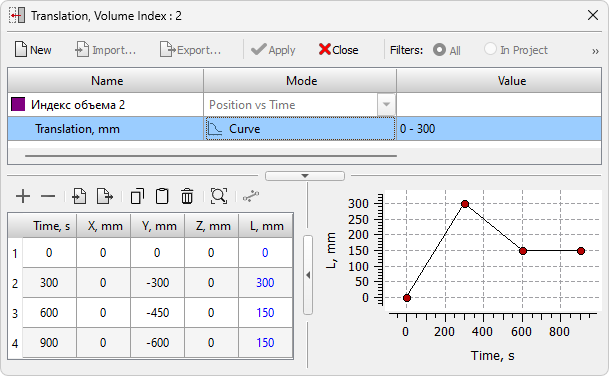
Translation mode for volumes with index 2
Often, translation is used when simulating vacuum casting in combination with radiation heat transfer (for more details, see the Radiation Heat Transfer section). Often, translation is used when simulating vacuum casting in combination with radiation heat transfer (for more details, see the “Radiation Heat Transfer” section). If translations are specified, a ray tracing calculation will be performed for each point in the graph, and linear interpolation between two adjacent times for all intermediate points in time will be used. For such calculations, you should specify the number of points necessary for a qualitative description of the visibility of objects during the entire calculation. But it should be remembered that a large number of points in the translation curve significantly slows down the calculation with radiation heat transfer.
All specified translation are displayed in the Translations tree on the Project Overview panel (see the figure below). They can be exported to a .pmov file by clicking the button (1) in the tree. This file can then be imported into another project by clicking button (2) (importing files of older versions with the mve extension is also supported). You can delete all movement modes or one selected mode using the button (3). The name for the translation modes can be specified in line (4), it is available for editing by double-clicking the left mouse button.
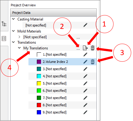
Translation tree in the Project Overview panel
Sliding Boundaries
The dialogue window “Sliding Boundaries” is dedicated for the creation and editing the files with the extension knt, having the information about the types of the sliding boundaries
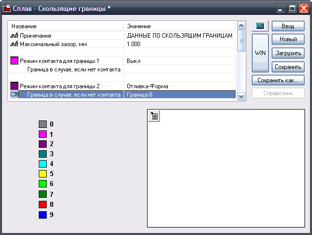
Sliding Boundaries Editor
The module “Furje-3D” of PolygonSoft system can work with the volumes having the mismatching meshes on the border. In this case it is necessary to create the file knt and to indicate the type of mismatching borders in it. It is necessary to do at the simulating the continuous casting when slab (foundry) moves through the crystallizer and intersection of the casting and mold meshes is broken at the beginning of the slab movement.
In this editor you should indicate it’s contact with the neighboring body for each interface with mismatching mesh. Double clicking on the “Contact mode for the boundary…” calls for drop-down list in which it is necessary to find the corresponding value and push the button “Enter” on the keyboard.
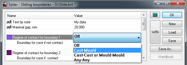
Selection of the mode of the contact for the border
The next line indicates which heat transfer parameters to assign, if the contact conditions have changed. Double-clicking on the left cell can bring up a list of conditions (see the figure below). There are two options:
- The boundary in case if there is no contact (by default). This condition works if the bodies have had the contact by the given boundary and at some period this contact has been lost (fully or partially) and the border became external. For example, the slab moves within crystallizer (there is the contact) and then a part of it appears outside the crystallizer within the zone of secondary cooling (the contact with the crystallizer is partially lost).
- The boundary in case if there is a contact. This is the opposite condition that starts to be active when there is the contact between the bodies by the given boundary (fully or partial). This condition is convenient to use, for example, when the slab passes different cooling zones with different heat exchange conditions with the medium, but some of its sections are in contact with the rollers and the conditions for heat transfer at the boundary "slab- rollers" are the same for all rollers.
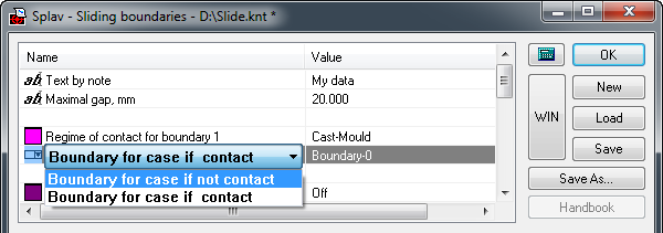
Selection of the condition with changing the contact
Having chosen the proper condition from the list, you should press the button “Enter” in the keyboard.
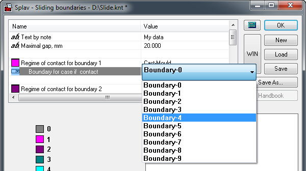
The chosen condition switches the heat transfer conditions. If the switching condition is not met, the heat exchange parameters for the specified boundary apply. If the switching condition is started, the heat exchange parameters set for any other boundary in the heat transfer file are switched. This "other" boundary is specified in the right cell of the line opposite the switching condition. Double-clicking on the cell opens the drop-down list of the boundaries (see the figure below), in which you need to select the desired option and press the "Enter" key on the keyboard.


 – radiation heat transfer coefficient.
 .
.
 ,
,
.svg)
.svg)
.svg)

.svg)