Criterial Analysis (Criterion Module)

The Criterion module is a post-processor of CSS PoligonSoft. The program is designed to create the static fields of scalar values - criteria calculated by the formulas supplied by the developers or created by the user, using the results of the heat simulation, previously performed by the Fourier solver, as the initial data. In the future, the created file of the criterial fields can be visualized using the Mirage module.

The module can be started from the CSS PoligonSoft shell with the Criterion button (see the figure below).

Start of the Criterion module

The interface of the Mirage module allows creating the functions for criterial analysis of the temperature, phase and other fields and processing the files with the simulation results by these functions.

Working window of the module

After the module is started, its working window is opened (see the figure below).

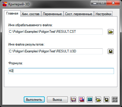
The working window of the “Criterion-3D” module

The window contains several tabs. On the “Main” tab, you specify the name of the file to be processed and the name of the results file. Also here you can load the file of the finished criterion and save the created or edited criterion.

	The button opens the standard file download dialog. With the help of it, you can upload any results files to the module. The name of the loaded file will be displayed in the field to the left of the button.
	The button opens the standard file saving dialog. Using it, you can specify the name and the location of the file with the result of the criterial analysis. The name of the file to be saved with the u3d extension will be displayed in the field to the left of the button.

A group of the buttons is located at the bottom of the window. Some of them are traditionally present in all modules of the system; the others are unique for this module.

	The button "Upload file with the formulas and settings" opens a standard dialog for loading a file with the extension cri. It contains the user-created criterial analysis functions and other module settings.
	The button "Save file with the formulas and settings" opens the standard file saving dialog. Using it, you can specify the name and location of the file with the created criterion and other settings of the module.
	The button "Show / Hide the button panel" opens an additional window for standard and ready criteria operations and functions. The information about them is found in the sections and "Available standard operations and functions" and "Available criteria variables and functions".

The tab "Chemical composition" is intended for those cases when the chemical composition of the alloy is included in the composition of the criterial formulas (see the figure below). This tab is almost equal to the next tab "Variables", but can be used separately.

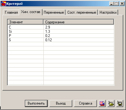
The tab “Chemical composition”

The tab "Variables" is intended for giving the values to the selected variables (see the figure below). The "Name" column is used to define the variables (or constants), in the "Value" column, the value of the variable (constant) is specified. To specify a change in the value when simulating this criterion, it is necessary to write down the formula that determines this change. The formula is written to the "Value" column in one line with the name of the variable specified in the "Name" column. If the value must be unchanged, a constant is entered in the “Value” column.

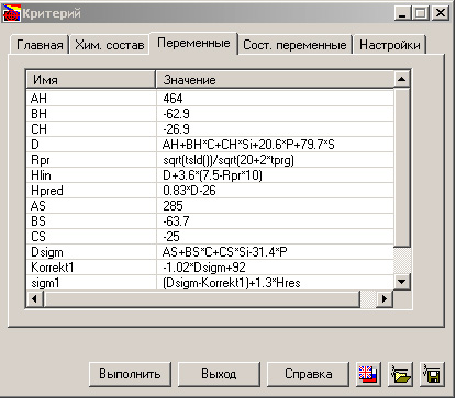
The tab “Variable”

When writing a formula, you can use the available standard criteria variables and the functions (their list is given in the section "Available criteria variables and functions" ), as well as the declared variables (constants).

ПWhen formulating a criterion, it often happens that it must be composed of several formulas. At the same time, this or that formula is applied depending on what value a variable has taken, depending on how large the processed values are, and so on. To take into account the possible branching in the computational scheme, the implementation of the transition in the simulations to one or another formula, the tab "Combined variables" is proivided regulating the state of the variables (see the figure below).

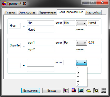
The tab “Combined variables”

On this tab, you can specify the logic of the transition from one variable (formula, constant) to another, using the "indicator" values of the variables that define the movement, entered in the movement conditions, composed using the mathematical symbols.

The last tab "Settings" (see the figure below). On this tab, when you can set the checkbox "Open the generated file in the "Mirage-3D” module. Upon completion of the simulation of the criterial function, the results file will be automatically opened in the "Mirage-3D" module.

Also on this tab, you can specify the file name with a list of the slides associated with the results of processing the computational fields by this criterion.

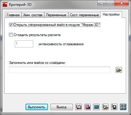
The tab “Settings”

Performing the simulation

After specifying the variables (the constants, the formulas) included in the criterion, and, if necessary, the transition logic, you can perform the simulation. In the "Formula" line on the "Main" tab, the user specifies the formula or variable described in the "Variables" tab. The values obtained in the simulation by this formula (or the value of the corresponding variable) will be displayed as a result. The simulation is started by clicking the "Run" button. After that, the program checks the correctness of the saved criteria, and then the simulation is performed, the results of which are written in *.u3d - file with the name specified on the "Main" tab.

In the case of an error in the writing the criterion, a message will be issued. The error can be in the syntax of the mathematical expressions (see the figure below)

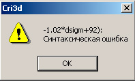
Error in the syntax of the mathematical expressions

or when using an variable in the formulas undeclared beforehand (see the figure below).

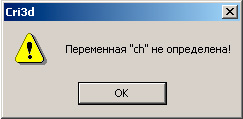
Ошибка необъявленной заранее переменной

The question of whether the formula of the criterion is correct from the point of view of the physics of the process and what information the field of this or that criterion will give is a theoretical question, and its consideration is beyond the scope of this description. When writing a formula, the user relies on his experience, on the information he has learned from the literary sources. You can also use the library of criteria developed by the developers.

In the process of simulating the criterion, there may be the computational errors associated with the peculiarities of the field values in the loaded results file. In this case, the module displays a corresponding message (see the figure below) and offers several options for further action.

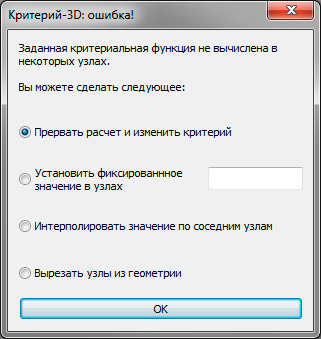
Error of simulating the criteria function

Interrupt the simulation and change the criterion. If you select this option, the criterion simulation will be stopped.
Set a fixed value in the nodes. If you select this option, you are prompted to enter a value in the field to the right that will be assigned to all nodes where the criterion simulation failed.
Interpolate the value of the adjacent nodes. In this case, the nodes where the criterion simulation has ended with the error will be assigned the values simulated according to the law of linear interpolation between the neighboring nodes.
Cut the nodes from the geometry. If you select this option, the nodes in which the criterion simulation failed, will be removed from the geometry.

It should be kept in mind that the appearance of such message does not always mean that the criterial function is composed incorrectly. For example, such situation can arise if the criterion simulates the cooling rate of the melt to the solidus temperature, but not all nodes have reached this temperature during the simulation of the thermal task.

Available standard operations and functions

The button "Show / Hide the button panel" opens an additional window of standard and ready-made criterial operations and functions (see below).

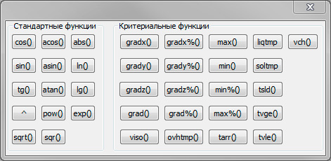
The panel of standard and criterial variables and functions

ИUsing the buttons of the panel, you can write these functions down in the variable tables on the corresponding tab. Below, a list of the functions and the variables available on the panel is given in this and the following sections.

+-/*	Standard arithmetic operations;
x^y	x to the power of y;
pow(x,y)	x to the power of y;
sqrt(x)	Square root of x;
sqr(x)	x squared;
abs(x)	Absolute value of x;
ln(x)	Natural logarithm of x;
lg(x)	Decimal logarithm of x;
exp(x)	Exponent from x;
sin(x)	Sinus x;
cos(x)	Cosine x;
tan(x)	Tangent x;
asin(x)	Arcsine x;
acos(x)	Arc cosine x;
atan(x)	Arc tangent x.

Available criterion variables and functions

Criterial variables
liqtmp	Liquidus Temp.*;
soltmp	Solidification Temp.*

Criterial functions
tsld()	Solidification time*, sec;
vch(val)	The rate of change of a value when it reaches the value val[%]**, units/sec;
tvge(val)	The time, during which the value is not less than the set value val[%]**, sec;
tvle(val)	The time, during which the value is not bigger than the set value val[%]**, sec;
gradx(val)	The x-component of the gradient at the moment of the variable reaching the value val[%]**, units/m
gradx%(val)	x-component of the gradient of the additional field * at the moment of the variable reaching the value val[%],units/m;
grady(val)	The y-component of the gradient at the moment of the variable reaching the value val[%]**,units/m;
grady%(val)	The y-component of the gradient of the additional field * at the moment of the variable reaching the value val[%],units/m;
gradz(val)	The z- component of the gradient at the moment of the variable reaching the value val[%]**,units/m;
gradz%(val)	The z-component of the gradient of the additional field * at the moment of the variable reaching the value val[%],units/m;
grad(val)	the complete (maximum) gradient at the time the value is reached val[%]**, units/m;
grad%(val)	the complete (maximum) gradient of the additional field * at the moment of the variable reaching the value val[%],units/m;
max()	Maximum value of the variable, units;
max%()	Maximum value of the additional *** variable, units;
min()	Minimum value of the variable, units;
min%()	Minimum value of the additional*** variable, units;
ovhtmp()	Overheating temperature*, Celsius degrees;
viso(val)	the velocity of the isosurface movement at the moment of variable reaching the value val[%]**, m/sec;
tarr(val)	time to reach the value val[%]**, sec.

* - the variables and the functions are available only for the casting temperatures files (*.cst)

** - if the functions argument ends by the symbol ‘%’, then the argument is decided to be the auxiliary field (for the files *.cst – the filed of liquid phase in the percent, for other types of the files it corresponds to the basic field).

*** - about the meaning of the “auxiliary field” – see the note **.

The examples of the criterial functions (for the file *.cst).

rad(liqtmp) – the gradient of the temperature field at the time when the temperature in the node is equal to the liquidus temperature
grad(50%) – the gradient of the temperature field at the time when the fraction of the liquid phase in the node is 50%.
grad%(liqtmp) – the gradient of the field of the liquid phases at the moment when the temperature in the node is equal to the liquidus temperature.
grad%(50%) – the gradient of the field of the liquid phases at the moment when the fraction of the liquid phase in the node is 50%.